Rates in detail

Chapter 1 introduced the shape every rate takes, effective rate = scope(base) × modifiers. This appendix is the full reference: how a rate's units work, the default scope at each level, the catalogue of modifiers and which levels accept them, and what the engine does with a rate once it has one.

How a rate is counted: the scope

A rate is a number of events per unit time, the time the species tree imposes, for one unit of whatever it is counted over. A substitution happens at a site, so a substitution rate is counted per site: each site is an independent chance to mutate. A speciation happens to a lineage, so the speciation rate is counted per lineage: each branch alive is an independent chance for the tree to split. A gene is lost one copy at a time, so gene loss is counted per copy. The unit a rate is counted over, a lineage, a copy or a site, is what we call its scope.

By default, this is the scope ZOMBI2 uses at each level:

Level	Counted per	The rates it applies to
Species	lineage	birth, death
Genomes, family and ordered	copy	duplication, transfer, loss
Genomes, family and ordered	lineage	origination
Genomes, ordered	copy	inversion, transposition, translocation
Genomes, ordered	chromosome	fission, fusion, chromosome_loss
Genomes, ordered	lineage	chromosome_origination
Genomes, nucleotide	lineage	duplication, transfer, loss, origination, inversion, transposition, translocation, chromosome_origination, insertion, deletion
Genomes, nucleotide	chromosome	fission, fusion, chromosome_loss
Sequences	site	substitution (times a clock)
Traits	lineage	rate (continuous), switch (discrete)

A bare number takes the default, and writing the default scope explicitly is accepted at every level. A discrete trait's switch also takes two shapes that are not a single rate: a {'from->to': rate} dict, whose values are rates in either spelling, and a k×k matrix, whose entries are plain numbers: every entry there is counted per lineage, so a cell has no scope of its own to write.

Three rows of that table accept a second scope, and each extra scope is a different model rather than a different spelling:

Rate	Also accepts	What that means
Species birth, death	Global	one budget for the whole tree: linear growth, not exponential
Genomes, family and ordered: duplication, transfer, loss	PerLineage	a fixed budget per lineage: the rate is the same however much the genome holds
Genomes, ordered: inversion, transposition, translocation	PerLineage	the same, for the rearrangements

The difference is large and worth stating plainly. loss = PerCopy(0.25) puts every copy independently at risk, so a genome of a thousand genes loses ten times as often as one of a hundred. loss = PerLineage(0.25) is a deletion budget: the lineage loses at 0.25 whatever it holds, and the genome's size never enters. The same number, and in the hundred-gene genome the two models sit a hundredfold apart.

origination stays per lineage, since it is the rate at which new families arrive and per copy it would be zero in an empty genome. The chromosome rates stay per chromosome. The nucleotide resolution already counts its gene events per lineage, which is why it has no second scope to offer: there the rate says how often a lineage does the thing and the extent says how much DNA it touches.

from zombi2 import species
from zombi2.params import Global

# a death rate applied to the whole tree at once, not once per lineage
species.simulate_species_tree(birth=1.0, death=Global(0.3), total_time=8.0, seed=2)

Global(x) detaches the rate from the amount of material present, so a Global death rate does not grow as the tree does. When a Global event fires, the lineage it lands on is drawn as always, weighted by the lineages' own factors, so uniformly among the living when nothing sets one apart. The scopes are Global, PerLineage, PerCopy, PerSite and PerChromosome, and nothing outside these two tables is accepted: a rate handed any other scope is refused, and the error names the scopes its level takes.

How a rate changes in context: modifiers

A modifier alters a rate in context. You might give a gene family a constant loss rate across the tree except in one clade known to shed genes, a symbiotic bacterium, by multiplying the rate there. Or let families evolve at different speeds: an antimicrobial-resistance family prone to transfer, a ribosomal-protein family the opposite.

The modifiers are:

Verb	What it does to the rate
changing_at	Follows a time schedule: one factor up to a breakpoint, another after it.
scaled_by(TotalDiversity(cap=...))	Slows as the tree fills up: the factor falls from 1 toward 0 as the number of lineages approaches a carrying capacity, and stays there.
varying_among('lineages', Drift(...))	Is inherited from the parent lineage and nudged at each split, so the rate drifts gradually down the tree and close relatives keep similar rates.
varying_among('lineages', ...)	Is an independent draw for each lineage, with no memory of its parent, so nearby branches are no more alike than distant ones.
varying_among('families', ...)	Is an independent draw for each gene family, so one family is prone to transfer and another is not, whatever lineage either sits in.
scaled_by(driver, mapping)	Depends on an evolved value: the factor is looked up from a driver's state, either another level or another run of the same one, which is how one thing conditions another (Chapter 8).
set_by(driver, mapping)	Replaces the base instead of multiplying it: the mapping gives the rate itself, in the rate's own units, so nothing is written in front of it. It takes a driver just as scaled_by does, the scope still applies, and a rate carries one.

The first two are deterministic: the clock and standing diversity are fixed functions of the state of the world, so every lineage that meets the same time, or the same diversity, gets the same factor. The next two are random and vary from lineage to lineage, and they differ in memory: a Drift law is passed down and drifts, so the rate is autocorrelated along the tree, a slowly wandering clock or a clade that inherits a fast tempo, whereas a bare distribution is drawn afresh on every branch, so the variation is scattered, an uncorrelated ("relaxed") clock. varying_among('families', ...) is the same independent draw made over gene families rather than lineages, so it varies what a family does wherever it sits. All three random laws are mean-corrected, meaning their factors average to 1, so a lineage is no likelier to be sped up than slowed down.

Be careful about what that does and does not buy you. It fixes the factor, not the tree. A birth rate that drifts is multiplicative, and a branching process is convex in its rate: the fast lineages branch, and their descendants inherit the fast tempo, so they come to dominate the tree while the slow ones contribute almost nothing. Standing diversity therefore rises as you widen the distribution, even though every individual factor averages to 1, and at moderate spread a run can grow explosively enough to hit the max_lineages guard. Mean-correcting keeps the rate honest per lineage; it does not hold E[N(t)] fixed, and nothing could.

Where a driver attaches. A driven factor is neither random nor corrected: it is whatever the driver's state says it is. A driver need not come from another level: Clade({"fast": ["n12", "n27"]}) names a subtree by its tips, or by a node id, and takes membership from the tree the run is already walking, with every unnamed lineage in "rest". A driver is not confined to a rate: the same factor multiplies an extent at the ordered and nucleotide resolutions, where an extent takes only changing_at and scaled_by: a per-family draw has no one family to read (a segment covers several), and set_by on an extent is not built. Drivers also go on transfer_to, written Recipients().weighted_by(driver, mapping) rather than scaled_by because there the numbers are normalised weights over the candidate recipients, compared against each other, with no base in front of them (Chapter 8). And TotalDiversity(cap=...) is written alone inside scaled_by, where a clade or a trait takes a mapping beside it, because it is driver and mapping in one: the standing count is the driver, and the falling curve is built in.

How wide the variation is, and what shape it takes. The law is varying_among's second argument, the distribution written out. Any built-in one works, so varying_among('families', Gamma(shape=4.0, scale=0.25)) gives the draws a gamma's shape and varying_among('families', LogNormal(0.0, 0.5)) the usual lognormal.

Read the law together with what wraps it, because the distribution describes a different quantity in each: written bare it is the value each unit gets, and inside Drift it is the step taken at every split, which accumulates down the tree. That is why there is no short spelling: a single spread=σ would have to name both quantities with one word, and could not say which distribution it meant. The built-in distributions are Fixed, Exponential, Gamma, LogNormal, Uniform and Geometric, all in zombi2.params.distributions.

Whatever the distribution, the draw is divided by its own mean, so what it contributes is its shape and not where it sits: Exponential(1.0) and Exponential(7.0) are the same law.

Drift takes one more, bins=. With it the value moves in steps rather than continuously: it takes one of bins values on a log-spaced ladder, and the step the law draws at each split, discretised, moves the daughter to a neighbouring rung or leaves it. The model is unchanged, only snapped to a grid. varying_among('lineages', Drift(LogNormal(0.0, 0.45), bins=6)) is the discrete-bin clock, where a clade's rate is one of a handful rather than anything at all.

Verbs chain, and their factors multiply, so they combine: PerLineage(1.0).changing_at({0: 1, 5: 0.3}) .varying_among('lineages', Drift(LogNormal(0.0, 0.3))) is a rate that both follows a schedule and drifts between lineages.

Which level accepts which

A modifier only makes sense where the level can act on it, and a level rejects one it does not accept rather than silently ignoring it. set_by is listed separately from scaled_by even though both take a driver, because replacing a base is a capability an engine has or has not: the three levels below can do it and the rest refuse. This is what each accepts today:

Level	The verbs it accepts
Species	changing_at · scaled_by(TotalDiversity(...)) · varying_among('lineages', Drift(...)) · varying_among('lineages', ...)
Genomes, family and ordered	changing_at · scaled_by · set_by · varying_among('families', ...)
Genomes, nucleotide	changing_at · scaled_by
Sequences	varying_among('lineages', ...) · varying_among('lineages', Drift(...)) · scaled_by
Traits, continuous rate	changing_at · varying_among('lineages', Drift(...)) · scaled_by(TotalDiversity(...)) · scaled_by · set_by
Traits, discrete switch	scaled_by
Joint, birth / death	changing_at · scaled_by(TotalDiversity(...)) · scaled_by

Each entry is written the way you would type it, with ... standing for the argument you choose, a distribution or a carrying capacity. The two varying_among entries are one verb and differ in their law: Drift(...) is the value inherited from the parent, a bare distribution the value drawn afresh.

zombi2 <command> -h lists a level's modifiers under "Modifiers this level takes", in these same words: the help is built from the level's own declaration, and a test checks this table against that same declaration, so neither can drift from it. Two commands each span two rows of the table: zombi2 genomes, whose nucleotide resolution reads fewer verbs than the other two, and zombi2 traits, whose --switch reads fewer than --rate. For those the help lists the larger row and gives the smaller in the note beneath it.

A modifier missing from a row is one that level does not read yet. It is not a claim that the combination would be meaningless; each engine gains a modifier when its own code learns to read it, and some have not got there. You never have to guess which: give a level a modifier it does not accept and the error names the ones it does, so this table can always be read back off the tool itself.

A state, but only after a time

scaled_by depends on a driver and changing_at follows the clock, and chaining them does not combine them: the factors multiply, and each applies to every lineage, so scaled_by(clade, {...}).changing_at({...}) puts the time window on the whole tree rather than on the clade.

To scope a factor to a driver state and to a time, write that state's entry as a schedule, in changing_at's own notation:

from zombi2.params import Clade, PerCopy

endo_loss = PerCopy(0.02).scaled_by(Clade({"endo": ["n76", "n112"]}),
                                    {"endo": {0: 1.0, 6.0: 20.0}, "rest": 1.0})

The endosymbiont clade loses genes at the base rate until t=6 and twenty times faster from then on, while everything outside it is unchanged throughout. The breakpoints are reported into the engine's horizon, the next-change stepping described under "When the rate changes with the clock", below, so the run steps to them rather than past them. Any discrete driver takes one too: a trait state whose factor changes at a time reads the same way.

The sequences level refuses a schedule inside a mapping. It walks each gene tree branch by branch and never steps at a wall-clock time, which is why changing_at is missing from its row above; a schedule there would hold its first factor for the whole run, so it is refused rather than half read.

Writing your own

The modifiers above are the ones ZOMBI2 ships. If none of them says what your rate depends on, you can write your own. It is a small class, and it needs two things.

A factor() method, returning the multiplier. The engine calls it as the run goes and hands it the context that engine has. Every engine passes time and lineages; the rest differ:

Engine	Context passed to factor
species	time, lineages, diversity
genomes.family	time, lineages, copies, drivers
genomes.ordered	time, lineages, copies, chromosomes, drivers
genomes.nucleotide	time, lineages, copies, chromosomes, drivers
traits.continuous	time, lineages, diversity, drivers
traits.discrete	time, lineages, drivers
joint	time, lineages, diversity, drivers

time is the run's clock and lineages the branches alive; copies and chromosomes are the lineage's own counts, and drivers carries the driven values a conditioned rate depends on. Take **_ and default every key you read. A key your engine does not supply never arrives, and the genome engines pass drivers only on a rate that is itself driven, so it can be missing even on an engine that lists it. One key is there and is always 0: copies at the nucleotide resolution, where gene events are counted per lineage rather than per copy, so there is no copy count to pass. What you return multiplies the rate, so 1.0 leaves it alone, 2.0 doubles it, 0.0 switches it off.

An implemented_for list, naming the engines that read it. A modifier an engine does not read would silently return 1.0 and hand you a run that is not the model you asked for, so a level takes only the modifiers that name it and refuses the rest. The engine names are species, genomes.family, genomes.ordered, genomes.nucleotide, traits.continuous, traits.discrete and joint.

Here is a complete one. TotalDiversity makes speciation slow down as lineages pile up. This makes extinction speed up instead, which is the other half of the same idea and something no shipped modifier can say:

from zombi2 import species
from zombi2.params.evaluate import Modifier

class OnCrowding(Modifier):
    """Extinction rises as lineages accumulate: at `crowd` standing lineages it has doubled."""
    implemented_for = ("species",)

    def __init__(self, crowd):
        self.crowd = float(crowd)

    def factor(self, *, diversity=0.0, **_):
        return 1.0 + diversity / self.crowd

That is the whole modifier. The verbs build the shipped ones, so there is no verb that attaches one of yours; build the rate from Rate instead, giving it the base, the scope class, and the modifiers in the order they should be drawn in:

from zombi2.params import PerLineage
from zombi2.params.parameter import Rate

plain   = species.simulate_species_tree(birth=1.0, death=0.2, total_time=6, seed=3)
crowded = species.simulate_species_tree(birth=1.0,
                                        death=Rate(0.2, PerLineage, (OnCrowding(crowd=50),)),
                                        total_time=6, seed=3)

print(len(plain.complete_tree.extant_leaves()))     # 290 lineages survive
print(len(crowded.complete_tree.extant_leaves()))   # 142 when extinction rises with crowding

Two limits. A modifier of your own is Python-only: --death and a --params file know the names ZOMBI2 ships and cannot build a class you wrote. And if your factor reads time, making it a rate that changes continuously rather than only when an event occurs, give the class a next_change(time) method returning the next moment the rate changes, so the engine stops and re-evaluates there instead of holding it at whatever it was, which is the same horizon stepping again. The modifiers are drawn in the order you list them: the factors multiply, so the product does not care, but draws consume the random stream in order, and that order is part of what the seed reproduces. OnCrowding needs none, because diversity only changes when something is born or dies, and the engine already re-evaluates then.

How a rate becomes an event

Almost every simulation here comes from one small engine, run over and over: the same loop grows a birth–death tree, duplicates and loses genes, and switches a discrete trait between states, given a different list of events each time. That engine is the Gillespie algorithm [@gillespie1976; @gillespie1977], an exact, event-by-event recipe for a continuous-time process defined by rates.

One pass of the loop is three steps. Add the rates of everything that could happen next, which gives the total rate. This sum is where the scope's arithmetic happens: a per-copy loss of 0.25 in a lineage of forty copies contributes 40 × 0.25 = 10, each copy its own independent chance, and a per-site rate counts its sites the same way. Draw one waiting time from an exponential with that total. The rate has no memory, so how long the run has already waited changes nothing. Then pick which event fired, each in proportion to its own rate, apply it, and start again from the state it left. Rates in, a timed history out. The derivation, why the waiting time is exponential and why the competing events can be raced this way, is a textbook one and is not repeated here.

When the rate changes with the clock

The loop above assumes the rates hold still between events, so that a single \(\text{Exponential}(R)\) draw lands exactly on the next event. That holds whenever the rates depend only on the current state, which changes only when an event occurs. But some rates move with the clock itself, even while nothing is happening: a changing_at schedule steps at fixed breakpoints, a scheduled mass extinction arrives at a set time, and a driven rate follows a driver that changes state on its own timetable. Now \(R\) is a moving target, and a draw at today's \(R\) would be wrong.

ZOMBI2 keeps the draw exact by never letting it cross a change. Every rate can report the next time it changes on its own, and the engine takes the earliest such time, together with the next scheduled pulse and the end of the run, as a horizon:

1. Compute \(R\) from the rates as they stand, and the horizon.
2. Draw \(\Delta t \sim \text{Exponential}(R)\).
3. If the event lands before the horizon, fire it: the rates really were constant over that stretch, so the draw is exact.
4. If it lands after, discard it, advance the clock to the horizon, and start again with the rates as they are there.

Discarding is sound for the same reason the loop works at all: the exponential is memoryless, so a partial wait carries no information into the next stretch. The rates are piecewise constant, each piece gets its own exact draw, and no integral or rejection step is ever needed.

What each level supplies

Each level that runs on events supplies its own list, and one loop realises them all; the two that do not are the next section's:

Level	The events	Their rates
Species	speciation, extinction	birth, death, per lineage
Genomes	duplication, transfer, loss, origination	one rate per event
Traits (discrete)	switches between character states	the entries of the switch matrix

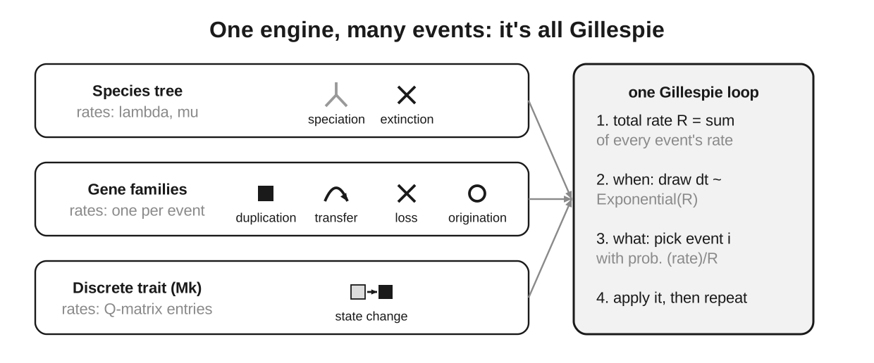
Swapping levels swaps the list of events and how their rates are computed; the timing machinery of total rate, exponential wait and proportional choice never changes.

Where the loop is not used

ZOMBI2 steps outside the event-by-event loop in two places, for the same reason both times: when only the endpoints are needed, not the whole timed history, an exact draw beats simulating events you would throw away. Neither is an approximation: both give the same distribution the loop would, in one step.

The first is sequence substitution along a branch. Once a gene tree and its branch lengths are settled, evolving a sequence down a branch does not require the individual substitution events, only the state at each end. The probability of ending in each state after a branch of length \(t\) is given exactly by the matrix exponential \(P(t) = e^{Qt}\), so ZOMBI2 draws each site's descendant state straight from \(P(t)\) in one step (Chapter 6). Running Gillespie here would generate, and then discard, thousands of intermediate substitutions. The exception is a run that asks for the history: record=True needs those substitutions, so it walks each branch event by event after all.

The second is a continuous trait. Brownian motion has no events to fire, since it moves at every instant, so there is nothing for the loop to enumerate. ZOMBI2 walks the tree branch by branch instead, in preorder, and draws one normal per branch: mean the parent's end value, variance the exact integral of \(\sigma^2\) along the branch (Chapter 7). With a constant \(\sigma^2\) that integral is just \(\sigma^2 \times\) branch length, and the values that come out have the Brownian structure exactly, variance \(\sigma^2 \times\) root-to-tip depth at a tip, covariance \(\sigma^2 \times\) shared path length between two, with no event drawn anywhere. The same walk serves OU, whose pull only changes which integral the branch draw uses, still exact, and the speciation jumps, one more exact draw at each split. A \(\sigma^2\) that varies along the branch changes only the integral, not the walk.

The rule of thumb is the same each time. Reach for Gillespie when you need the whole history, every branching, gain and loss at its exact time; reach for a shortcut when the endpoints are all you need. For the trees and genomes that are ZOMBI2's real subject the history is the result, so the loop is the norm and these two shortcuts are the exceptions.

Paths on Windows

ZOMBI2's test suite runs on Windows on every change, so the same command does the same thing there. Two things differ and are worth knowing before they bite:

• Paths in a rate expression. A driver path goes inside the rate. On the command line ZOMBI2 reads the backslashes as written, so PerCopy(0.25).scaled_by('C:\Users\me\trait_events.tsv', {...}) works as pasted. In a Python script the same line is Python source, and Python reads \U as an escape, so it is a SyntaxError. Worse, C:\temp is read quietly as C: followed by a tab. Write the path as a raw string there: r'C:\Users\me\trait_events.tsv'. Forward slashes work in all three places, the command line, a Python script and a --params file, and Windows accepts them.
• Paths in a --params file, the TOML file that can carry a run's flags (--params run.toml). TOML, not ZOMBI2, reads that file, and TOML's ordinary "…" string treats a backslash as an escape, so C:\Users fails there with a message about a hex value. Put a value containing a path in a TOML literal string instead, '''…''', which is taken exactly as written:

transfer-to = '''Recipients().weighted_by('C:\Users\me\trait_events.tsv', {'competent': 2.0})'''