Genomes III: nucleotide
At the nucleotide resolution a chromosome is a coordinate axis of DNA rather than a list of gene tokens, and events have an extension measured in base pairs: an inversion reverses 600 bp, a loss deletes 900 bp, a duplication copies 2 kb in tandem. Genes still exist and still get gene trees, but they are stretches of that axis with a start and an end, and the DNA between them is simulated too. The coordinates are the whole content: letters only exist once a sequence run reads the genome (Chapter 6), from a FASTA you supply or from a random sequence.
Genes and intergenes
A genome here is DNA, and its DNA is of two kinds:
- a gene is declared and indivisible: one family, one id, never cut in two. It carries a gene tree.
- an intergene is the spacer between genes. Nothing protects it, so events cut it wherever they land.
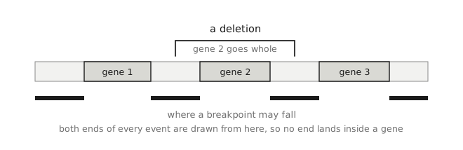
An event either engulfs a gene whole or leaves it alone; a breakpoint never falls strictly inside one. So an event does not pick a stretch and then clean up afterwards. Both of its ends are drawn directly from the positions where a breakpoint is legal. A genome can therefore be all gene, with no spacer at all: ten 100 bp genes in 1000 bp is a legal genome, and it evolves.
Extents
Indivisible genes have one consequence to meet before the rates: the realised extent is not always the extent you asked for. An event covers an arc, the stretch of DNA it takes, and both ends of an arc must fall where a breakpoint is legal. The draw is therefore the distribution you asked for, restricted to the ends that exist; nothing is drawn and rejected, so no event silently vanishes. Take thirty-one 3000 bp genes in a 100 kb genome, 93% genic, so the spacers are about 200 bp, and ask for an inversion of:
| asked | mean realised |
|---|---|
| 500 bp | 100 |
| 1 500 bp | 1 022 |
| 3 000 bp | 2 506 |
| 10 000 bp | 9 329 |
Means over about 1,500 inversions each. A 500 bp request has mostly spacer to land in, so the typical event collapses into one, with a median under 40 bp, while the occasional arc that spans a whole gene pulls the mean up to 100. Long requests can take genes whole, so they land near what you asked. The correction runs the other way too: on the all-gene genome above, the joins between genes are the only legal ends, so a 5 bp request comes out at 100 bp, a whole gene. Either way the event still happens: an extent is a request, and the run takes the closest arc the legal breakpoints allow. The one case that yields no event is a replicon with no legal end at all, such as one under 2 bp, where the event is skipped rather than forced.
A note on rates
Every rate here is per lineage. The rate sets how often a lineage does the event; the extent (above) sets how much DNA it touches. Keeping the rate per lineage means the number you type reads the same whatever the genome's size: a rate counted per base pair would rise as the genome grew, so inversion=5.0 would mean one thing at 10 kb and another at 1 Mb. Per lineage, the event count stays flat as the genome grows. The same tree at inversion=5.0, with the genome ten times longer each row, gives:
The chromosome rates are the exception: fission, fusion and chromosome_loss are counted per chromosome, and chromosome_origination per lineage. A fusion joins two chromosomes of the same topology, for the same reason it does at the ordered resolution: a ring and a molecule with two ends cannot become one molecule.
Insertions and deletions
Two more events move DNA without touching the gene inventory, the indels:
deletionremoves an arc, aslossdoes, but no copy lineage ends: the material goes, and every gene keeps its place in the genealogy.losschanges what a lineage has, because copies die and a gene can go whole;deletionchanges how much of a surviving stretch it carries.insertionlays down a stretch of novel spacer, asoriginationlays down a new gene:originationbrings a gene family into the run,insertionbrings sequence, DNA that descends from nothing.
In practice the difference is one of scale, and the extent defaults say so: 50 bp for the ancestry-changing events, 5 bp for the indels. Appendix B says where each is written: deletions in their own record, insertions as roots of their own kind.
Reading a genome, block by block
Two leaves of an inversion run show what its events did. describe writes one out: each line is a block, a stretch of DNA with one unbroken ancestry, written as the interval it came from on the initial sequence, read forward (+) or reverse-complemented (−). A gene is always one block, because nothing may cut it. Spacer is not, so several intergene lines in a row are simply spacer that has been cut apart and rearranged: the accumulated breakpoints of everything that happened to that lineage.
from zombi2 import species, genomes

tree = species.simulate_species_tree(birth=1.0, death=0.1, n_extant=4, seed=56)
g = genomes.simulate_genomes_nucleotide(
    tree, root_length=3000, genes=3, gene_length=400,
    inversion=1.0, inversion_extent=600, seed=56)

print(g.describe(2))
print(g.describe(5))
n2, chromosome 2
  [   0, 600) +  600 bp  intergene
  [ 600,1000) +  400 bp  gene 1
  [1000,1140) +  140 bp  intergene
  [2000,2065) −   65 bp  intergene
  [1600,2000) −  400 bp  gene 2
  [1573,1600) −   27 bp  intergene
  [1410,1573) +  163 bp  intergene
  [1140,1410) −  270 bp  intergene
  [2065,2563) +  498 bp  intergene
  [2563,2596) −   33 bp  intergene
  [2596,2600) +    4 bp  intergene
  [2600,3000) +  400 bp  gene 3
n5, chromosome 5
  [   0, 512) −  512 bp  intergene
  [2600,3000) −  400 bp  gene 3
  [2532,2600) −   68 bp  intergene
  [ 512, 600) +   88 bp  intergene
  [ 600,1000) +  400 bp  gene 1
  [1000,1600) +  600 bp  intergene
  [1600,2000) +  400 bp  gene 2
  [2000,2532) +  532 bp  intergene
Both leaves still carry all three genes, and both are still 3000 bp. In n2 an inversion covered gene 2, which now reads on the − strand with the spacer around it reversed; in n5 a different inversion covered gene 3 instead, taking the spacer on either side of it with it. The coordinates are what make this readable: every block still names where it came from on the initial sequence, so [600, 1000) is gene 1 wherever it turns up and whichever way it points.
The initial genome
The initial genome, the genome the run starts from at time 0 before any event, is declared in one of two ways. (It is not the same as the genome at the root node: the root branch is real simulated time, so that one already carries stem events. See .initial_genome in Appendix B.)
Evenly spaced genes. root_length=L sets each replicon's length in base pairs, and genes=N, gene_length=l lays down N genes of l bp on each replicon, spreading the leftover DNA evenly between them. The karyotype is chromosomes=: an integer makes that many equal replicons of root_length each, "circular" by default or topology="linear"; a list of (length, topology) pairs makes them unequal. Good for controlled experiments, since gene density is then a number you set.
A GFF file. gff="genome.gff" takes exact coordinates from a real annotation. ##sequence-region gives each replicon's length, gene features give coordinates, strand and name, and other feature types are ignored. Names land in result.gene_names, so you can follow a named gene through the run. gff= and genes= are mutually exclusive; a GFF already declares the genes (Ge11). Genes may touch but never overlap, since a gene is one indivisible block. Real annotations do overlap, usually by a base or two where genes abut in an operon, so an overlap is refused rather than guessed at: trim_overlaps=True (--trim-overlaps) pushes each overlapping gene's start to its neighbour's end instead, and drops any gene swallowed whole.
A genome at this resolution is rebuilt rather than stored: the run keeps the root partition, the initial sequence cut at every breakpoint any lineage ever used, and how each node's genome is assembled from those pieces, which is what keeps a million-base genome down a large tree affordable. Appendix B names both (.root_blocks, .assembly).
A GFF gives coordinates, not letters. fasta="genome.fasta" supplies the DNA those coordinates hold, one record per replicon, matched by id and each exactly its declared length, and a later zombi2 sequences run founds its blocks from that DNA (Chapter 6).
On the command line
--resolution nucleotide takes the same event rates as Chapter 4 and adds two things: how to set up the initial genome, and how long an event is in base pairs.
# an evenly spaced initial genome: 5 kb, six 300 bp genes, inversions averaging 400 bp
zombi2 genomes out/ --resolution nucleotide \
  --root-length 5000 --genes 6 --gene-length 300 \
  --inversion 1.0 --inversion-extent 400 --duplication 0.3 --loss 0.3 --seed 1

# or start from a real genome: the GFF declares the replicons and the genes,
# and a paired FASTA supplies the actual DNA those coordinates hold
zombi2 genomes out/ --resolution nucleotide \
  --gff ecoli.gff --fasta ecoli.fasta \
  --inversion 0.5 --loss 0.4 --loss-extent 900 --seed 1
Every event kind has its own --<event>-extent, the mean of a geometric draw in base pairs, 50 bp unless you set it and 5 bp for the indels: --inversion-extent, --loss-extent, --duplication-extent, --transfer-extent, --transposition-extent, --translocation-extent, --origination-extent (the length of the new gene an origination lays down), --insertion-extent, --deletion-extent.