Trait evolution

The trait level evolves phenotypes: a body size, a habitat, the presence or absence of a structure. A trait evolves along the species tree like everything else here. There are two kinds, continuous and discrete:

from zombi2 import species, traits
from zombi2.rates import modifiers as mod

tree = species.simulate_species_tree(birth=1.0, death=0.3, n_extant=20, seed=1)
result = traits.simulate_continuous(tree, start=0.0, rate=1.0, seed=1)   # a real value
result = traits.simulate_discrete(tree, states=["marine", "terrestrial"],
                                  switch=0.1, seed=1)                     # a discrete state

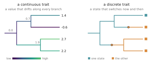
Continuous traits

A continuous trait does Brownian motion. Give it a starting value and a diffusion rate and it wanders down every branch, its variance growing in proportion to elapsed time:

# BM — a body size diffusing from 0 at variance-rate σ² = 1.0
traits.simulate_continuous(tree, start=0.0, rate=1.0, seed=1)

Here rate is the Brownian variance-rate σ², the trait level's reading of "how fast", and like every rate in ZOMBI2 it accepts modifiers. For example, two variations on this are:

# OU — the same diffusion, pulled toward an optimum value
traits.simulate_continuous(tree, start=0.0, rate=1.0,
                           reverts_to=2.0, pull=0.5, seed=1)

# early burst — the diffusion rate itself decays through time
traits.simulate_continuous(tree, start=0.0,
                           rate=1.0 * mod.OnTime({0: 1.0, 5: 0.2}), seed=1)

The Ornstein–Uhlenbeck process is Brownian motion with a rubber band: reverts_to is the optimum it is pulled back toward, and pull is how hard. Early burst (or ACDC) is a diffusion rate that decays as the tree ages, so most of the divergence happens near the root; it is written with the same mod.OnTime that gives the species tree its skyline.

The rest of the modifier vocabulary applies to rate unchanged, each with a name in the comparative-methods literature: mod.FromParent(spread=…) makes σ² drift from parent to daughter (variable-rates BM, the trait twin of ClaDS), mod.OnTotalDiversity(cap=…) slows σ² as the clade fills. Two knobs sit alongside rate: regimes= paints a multi-optimum OU, where clades pull toward different optima (a discrete trait supplies the painting and reverts_to becomes one optimum per regime), and at_speciation= adds a jump at each split rather than along the branches.

Discrete traits

A discrete trait takes a finite set of states and switches between them along the branches — a continuous-time Markov chain, the field's Mk model:

# Mk — habitat flips between two states at rate 0.1
traits.simulate_discrete(tree, states=["marine", "terrestrial"],
                         switch=0.1, start="marine", seed=1)

When the flips are not symmetric, replace the single rate with a small matrix of directed rates:

# asymmetric — gains are commoner than losses
traits.simulate_discrete(tree, states=["absent", "present"],
                         switch={"absent->present": 0.2, "present->absent": 0.05},
                         seed=1)

A threshold trait is the third case, and it is a bridge back to the continuous world. An observed discrete state can be driven by an underlying continuous liability that itself does Brownian motion; the state you see is which side of a threshold the liability currently sits on:

# threshold — a discrete state read off an underlying continuous liability
traits.simulate_discrete(tree, states=["absent", "present"],
                         liability=1.0, threshold=0.0, seed=1)

Correlated traits

Two traits that evolve independently are two separate calls, in either order. Two traits that drift together cannot be simulated one before the other, because each is entangled with the other as it unfolds. Correlation is specified as per-trait rates plus a correlation overlay:

traits.simulate_continuous(tree,
    start={"size": 0.0, "limb": 0.0},
    rate={"size": 1.0, "limb": 0.8},        # one variance-rate per trait
    correlation={("size", "limb"): 0.6},    # the overlay, ∈ [−1, 1]
    seed=1)

The overlay is a dimensionless number in [−1, 1], not a covariance matrix. Under correlation= the per-trait rates are plain numbers.

The same overlay handles discrete correlation with no extra machinery, through the threshold model: give each trait a liability, correlate the liabilities, and put the thresholds on top. Correlated presence/absence characters, the setting Pagel's method was built for, are then one call:

traits.simulate_discrete(tree, states=["absent", "present"],
    liability={"wings": 1.0, "flight": 1.0},
    correlation={("wings", "flight"): 0.7}, threshold=0.0, seed=1)

Models from the literature

Trait models arrive under a thicket of names, and a reader who wants "an OU model" or "a threshold model" should be able to find it. The names live here, in one table, and organise nothing else in the chapter.

What it does	ZOMBI2	From the literature
a value diffusing	simulate_continuous(rate=…)	Brownian motion (BM)
diffusion pulled to an optimum	simulate_continuous(rate=…, reverts_to=…, pull=…)	Ornstein–Uhlenbeck (OU)
diffusion rate decays through time	simulate_continuous(rate=1.0 * mod.OnTime({…}))	Early burst (EB / ACDC)
diffusion rate drifts between lineages	simulate_continuous(rate=1.0 * mod.FromParent(spread=…))	Variable-rates BM
diffusion rate slows as the clade fills	simulate_continuous(rate=1.0 * mod.OnTotalDiversity(cap=…))	Diversity-dependent / ecological limits
the optimum differs between painted clades	simulate_continuous(regimes=…, reverts_to={…}, pull=…)	Multi-optimum OU (OUM)
the value jumps at each split	at_speciation=… (either kind)	Cladogenetic / punctuational change
traits evolving together	one simulate_continuous(rate={…}, correlation={…}) call	Multivariate BM
a discrete state switching	simulate_discrete(states=…, switch=…)	Mk (k-state Markov)
discrete driven by continuous liability	simulate_discrete(liability=…, threshold=…)	Threshold / liability (Wright–Felsenstein)
discrete traits evolving together	simulate_discrete(liability={…}, correlation={…})	Correlated binary / Pagel

The objects

A run returns a TraitsResult bundle:

• .values — the observable vector: the trait's value at each extant tip. This is the comparative-data matrix a method would be handed.
• .node_values — the value at every node (extant, extinct, and internal alike), the true ancestors at each split, from the same process that produced the tips.
• .events — the timestamped event log, the same shape as the genome level's: each entry is a change on a lineage at a time, from one state to another, and its kind is on_branch (a switch along a branch) or on_speciation (a jump at a split). For a discrete trait this log is the source of truth. A continuous trait diffuses with no along-branch events, so its log holds only the at_speciation jumps and is empty without them.
• .history — for a discrete trait, the per-branch stochastic character map derived from that log: the ordered list of (state, duration) segments each branch passed through. It is None for a continuous trait, which has no map, and for a threshold trait, whose liability crossings are un-timed.

For discrete traits the stored values are the state labels you gave (not integer indices), so .values and .node_values already read back in your own vocabulary.

Usage from Python

from zombi2 import species, traits
from zombi2.rates import modifiers as mod

# a species tree from the previous chapters, then a trait riding along it
# (the complete tree — a trait evolves on extinct lineages too)
tree = species.simulate_species_tree(birth=1.0, death=0.3, n_extant=30, seed=1).complete_tree

# continuous: body size under Brownian motion
size = traits.simulate_continuous(tree, start=0.0, rate=1.0, seed=1)
size.values                 # {extant tip: float}

# continuous: an Ornstein–Uhlenbeck trait pulled toward an optimum of 2
temp = traits.simulate_continuous(tree, start=0.0, rate=1.0,
                                  reverts_to=2.0, pull=0.5, seed=1)

# discrete: habitat flipping between two states
habitat = traits.simulate_discrete(tree, states=["marine", "terrestrial"],
                                   switch=0.1, start="marine", seed=1)
habitat.values              # {extant tip: "marine" | "terrestrial"}
habitat.events              # the realized flips, in time order

# two continuous traits that drift together — one joint call
bodyplan = traits.simulate_continuous(tree,
    start={"size": 0.0, "limb": 0.0},
    rate={"size": 1.0, "limb": 0.8},
    correlation={("size", "limb"): 0.6}, seed=1)

Usage from the CLI

The state space is --kind, and it is required. It decides which of the other flags apply — --rate and the OU knobs belong to a continuous trait, --states and --switch to a discrete one — so there is no default that would not silently pick a model for you:

# a continuous (Brownian) trait along a species tree
zombi2 traits out/ --kind continuous \
    --start 0.0 --rate 1.0 --seed 1

# a discrete two-state trait
zombi2 traits out/ --kind discrete \
    --states marine,terrestrial --switch 0.1 --seed 1

# the same, also writing the driver file a conditioned genome run reads (Chapter 9)
zombi2 traits out/ --kind discrete \
    --states cave,surface --switch 0.1 --seed 1 \
    --write values events tree

The trait evolves on the complete tree, extinct lineages included, so species_complete.nwk is the file to hand it. An external tree works too; if it is not ultrametric you must declare each tip's fate with --tip-fates, because ZOMBI will not guess which early-ending tips are extinct.

Outputs

A run writes the trait values at the extant tips (trait_values.tsv, the observable comparative-data vector) and the trait tree (trait_tree.nwk, the complete tree with every node annotated [&trait=…], which opens in FigTree or iTOL). Because the value at every node comes from the same process that produced the tips, that annotated tree carries the exact ancestral states, not a reconstruction.

For a discrete trait the command also writes the event log (trait_events.tsv): a root row giving the state at t=0, then every realized transition with its time — the ground truth against which an ancestral-state or stochastic-mapping method would be scored. That one file is also what a conditioned genome run reads to let a trait drive its rates: given the shared tree, the root state plus the switches reconstruct the trait on every lineage at every instant, so no separate driver file is needed. The full list of files lives in Appendix B.