Dependent runs
The book has so far run the levels one at a time: a species tree first, then genomes on it, then sequences, then traits. This order exists because each level needs the previous one: a genome evolves along the species tree, and a sequence evolves inside a gene of the genome.
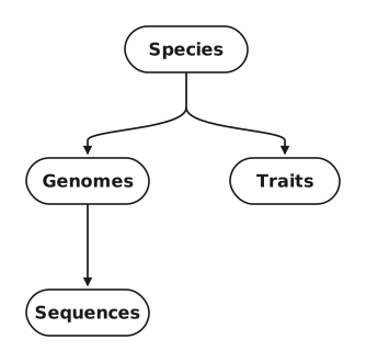
Sometimes you want to create more complex evolutionary scenarios, for example:
- A trait controls how quickly genes are duplicated.
- A gene controls how quickly a different gene is lost.
- The GC content of an organism controls one of its traits.
- A trait controls how quickly lineages speciate, and the trait evolves along the tree that it shapes.
- The composition of a gene controls how quickly its genome loses genes, and the genome controls which copies of that gene exist.
In all these scenarios, one simulation depends on another. This chapter first distinguishes the three kinds of run, then explains the connection, which is how every dependency is written, and finally presents the joint models.
Independent, conditioned and joint runs
There are three possible relations between two simulations.
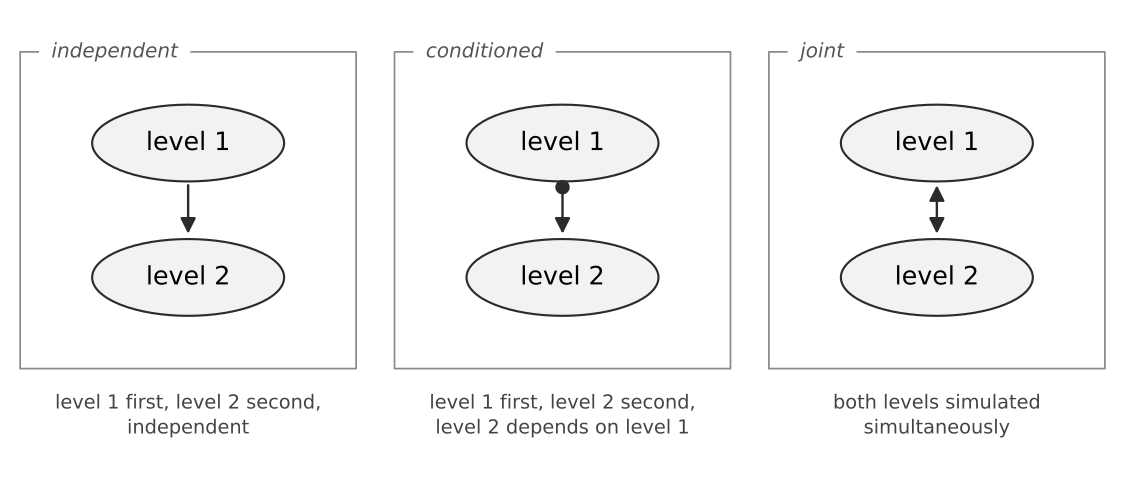
In an independent run the levels are simulated one after the other. The second simulation runs along the output of the first, a genome along the species tree for example, but its parameters do not depend on what happened in the first run. Every run in the previous chapters was of this kind.
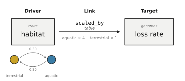
In a conditioned run the levels are also simulated one after the other, but the parameters of the second run depend on the results of the first. A habitat trait is simulated first, and the loss rate of the genome run then depends on the habitat of each lineage. In Python, the result of the first run is passed to the second as an object. On the command line, the second run reads the file that the first run wrote. The second run records what it depended on in a conditioned_on file (Appendix B), and re-running the driver afterwards requires --force, so the runs that depend on it cannot be left out of date silently.
In a joint run the two levels are simulated at the same time, in a single run. This is necessary when neither level can be simulated first, and there are two ways it happens. The first is a cycle of two connections: a trait controls the substitution rate of a gene, and the composition of that gene controls how the trait changes, so each simulation would need the other one to be finished. The second is a single connection that points against the normal order of the levels: the composition of a gene controls the loss rate of its genome, but the genome must be simulated to know which copies of the gene exist. In both cases there is no possible order, so one run simulates both levels.
A dependency is always created by a connection. A joint run without any connection is refused: without a dependency the result would be identical to two independent runs, and the error message says to run them independently instead.
Connections
Every dependency in this chapter is written in the same way, whatever the levels involved and whether the run is conditioned or joint.
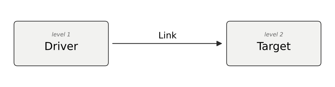
A connection has three parts. The driver is the value the connection takes as input: the state of a trait, the presence of a gene family, the GC content of a gene. The target is the parameter that depends on it: a loss rate, a substitution rate, a speciation rate. The link is what joins them: it states what number each value of the driver produces, and what that number does to the target.
The driver
A driver can be the state of a discrete trait, the value of a continuous trait, the presence of a gene family, the completion of a module, or the composition of a sequence. Appendix C lists them all, with what each one offers and a gallery example.
A driver is evaluated wherever it changes, not once per branch. A lineage that switches habitat halfway along a branch loses genes at one rate before the switch and at another after it (Co4). A discrete driver changes at specific moments, and the run steps to them exactly. A continuous driver changes all the time, so it is sampled every step of time instead, an argument written on the link: scaled_by(size, Curve(...), step=0.01). On the sequence level, where a driven rate becomes a branch length, the factor is integrated along the branch across the driver's changes.
A continuous trait is recorded only at the nodes, so what it did between two of them has to come from somewhere. ZOMBI2 draws it: the trait's path along the branch, conditioned on the value at each end. The path is drawn after the trait is simulated, from its own stream, so the trait's node values are the same numbers whether or not anything reads the path. Write path=False on the link to read the straight line between the two node values instead. The line is that path's average, and averaging first is not the same as reading a curve: under a mapping like exp, the line gives a rate that is too low, and halving step does not fix it because the line does not move. A run writes its path to trait_path.tsv, so a driver read from a file gives the same answer as the same driver held in memory.
In a conditioned run, a trait driver works both from Python and from the command line, where it is read from the trait's event file. The genome and sequence drivers (a presence, a completion, a composition) are objects in memory and work from Python only. A composition driver must also declare absent=, the value used on lineages that carry no copy of the family. Without it the run raises an error, because using the parent's last value would treat the family as still present, and that is a different model (Co20).
The target
A target is a parameter that would otherwise be a plain number: a rate, an extent, the recipient rule of transfers, or the substitution model of a sequence. In Python it is a keyword argument, on the command line a flag. Each level accepts only its own targets, and refuses a driven parameter it does not have. The targets are the rates of every level: the four rates of a family genome and a declared family's own rates, the eleven rates of an ordered genome, the thirteen of a nucleotide one, and their extents, the substitution rate of a sequence, the rate or switch of a trait, and, in joint runs only, the birth and death rates of the species tree. Two targets are not rates: transfer_to, the choice of a transfer recipient, and the substitution model of a sequence run. The full table is in Appendix C.
The link
A driver and a target have different units. A habitat is aquatic or terrestrial; a loss rate is a number of losses per copy per unit of time. The link converts one into the other, and it has two parts: the mapping states what number each value of the driver is worth, and the verb states what that number does to the target.
This line defines the loss rate of a genome run: a base rate of 0.25 per copy, multiplied by 4 in aquatic lineages. scaled_by is the verb and the dictionary is the mapping, and these are also the names of the arguments: scaled_by(driver, mapping).
There are three verbs. scaled_by multiplies the base rate and also applies to extents. set_by replaces the base rate, and its mapping then gives the rate in its own units. weighted_by applies to transfer_to and weighs the candidate recipient lineages against each other.
There are four mappings, and the right one depends on the driver. A Table gives one factor per state of a discrete driver. A Curve is a function of a numeric driver. A Scalar gives the factor exp(strength × value). A Between gives one weight per pair of donor and recipient states, for transfers only. The factor that comes out of a mapping is a number without units and cannot be negative. Appendix C gives both tables, with their rules and the gallery examples.
What can connect to what
Not every pair can be connected. A genome cannot be driven by a second genome run of the same lineage, because one genome per lineage is the model. A sequence can drive the genome that carries it, but only in a joint run: the genome must be simulated to know which copies of the sequence exist. The species tree can only be a target of joint runs, because no level can be simulated before the tree it evolves along. The full catalog is in Appendix C: a map of the pairs, and the table of every connection with the gallery examples that run it conditioned or joint.
Joint runs
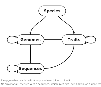
Levels can also be simulated jointly, as the figure shows. Two pairs reach the species tree: a trait or the gene content drives speciation, and the tree is then a result of the run. Three pairs join two different levels along a tree used as input: a trait and a genome, a trait and a sequence, a genome and a sequence. In the remaining three cases the two joined parts belong to the same level: a gene family changes the rates of the genome that carries it, one trait changes how another trait evolves, and each of two genes changes how fast the other one evolves. A joint run holds exactly two parts, and asking for a third is refused. The species tree and a sequence cannot be joined: a sequence evolves along a gene tree, which evolves along the species tree, so joining the two would require simulating the genome as well.
Naming the driver
The connections of a joint run are written with the same verbs and mappings as everywhere else. The difference is the driver. It cannot be passed as a finished result, because it does not exist yet, so it is named instead: "trait", "genomes:toxin", "sequences:rpoB". The name refers to another level of the same run, and the run grows both together. A run with a single trait can call it plainly "trait"; names exist so that a run can hold two. Appendix C lists the named drivers and what each one offers.
A family whose presence drives must be declared in the genome spec, with families=[family("toxin")]. On a tree passed with tree=, a declared family can also have its own duplication, transfer and loss, and these rates can read the other level of the run: with family("A", loss=PerCopy(0.3).scaled_by("trait", {"on": 6.0, "off": 1.0})), A is lost six times faster where the trait is on. A run that simulates the tree reads only the family's name. A gene whose composition drives a rate must declare it with offers=composition("KR", absent=0.02): which letters are counted, and the value used on lineages that carry no copy. A gene that drives a rate usually also declares start=, a second substitution model whose stationary frequencies are used only to found the gene. The gene starts with that composition and then evolves under its own model, so its composition moves toward its own equilibrium. Without start= a gene is founded at its equilibrium, its composition barely changes, and the rate that depends on it stays constant (Jo2).
A joint run is written from the specs of the levels it simulates, for example joint.simulate(species.birth_death(...), traits.discrete(...)). If the species spec is present, the tree is simulated, and the stop condition (n_extant=, total_time=) is written on that spec; if it is not, the tree is passed with tree= and the run ends where the tree ends. The result is a JointResult that carries both simulated levels, the same result objects the ordinary functions return, and both levels write their usual files. When the two joined parts belong to the same level, the run stays on that level's own function, with joint=True: simulate_traits, simulate_genomes_family or simulate_sequences. The flag is checked both ways: asking for it without a live driver is an error, and depending on a live driver without it is an error. One more restriction: a transfer needs the set of lineages alive at an instant, which is unknown while the tree is still being simulated, so a genome run that grows the tree refuses transfer. The gallery presents every joint model in full, with its code (Jo1 to Jo14).
Exact or sliced
A joint run advances by racing every possible event against every other, with the same Gillespie algorithm as everywhere in ZOMBI2. A discrete driver changes only at events, so between two events every rate is constant and the race is exact. When a speciation fires, it uses the trait state of the lineage it happens on; when a trait switches, the tree is untouched; both daughters of a split start from the parent's state.
Two kinds of driver change between events: a continuous trait diffuses at every instant, and a composition moves with every substitution. There is no interval over which the driven rate holds still, so there is nothing exact to race. These models slice time instead. Time is cut into steps of step, and the driver is held fixed within each slice, so the rates are constant inside it. At the slice boundary the driver moves: a diffusing trait by its exact transition law, a composition by the substitutions that accumulated. The approximation is only in the timing: the target uses the value the driver had at the start of the slice.
| Model | Tree | Advances by |
|---|---|---|
| a trait drives speciation | simulated | events, exact |
| gene content drives speciation | simulated | events, exact |
| a diffusing trait drives speciation | simulated | slices of step |
| a trait and a genome | input | events, exact |
| two discrete traits, each driving the other | input | events, exact |
| a continuous trait and another trait, each driving the other | input | slices; the driver is taken at the start of the slice |
| a trait and a gene's sequence | input | slices; the composition is taken at the start of the slice |
| a genome and a gene's sequence | input | slices; the composition is held within a slice |
| a gene family drives its own genome | input | events, exact |
| two genes, each depending on the other | input | slices; both compositions held within a slice |
step is written on the link, because the right size depends on how the value is taken: a steep curve needs a finer step than a flat one. In a joint run it has no default, and leaving it out is an error, because the timescale belongs to a model that does not exist yet.
A sliced run is first order in step: halve step and the error halves. Halving step also changes the numbers for a given seed, because it changes how many draws the run takes. The two runs are samples from two nearby laws, not one answer computed twice, so comparing them tells you nothing. Check convergence across seeds instead (Jo14):
- pick a summary the model is about — the mean value at the tips, the variance at the tips, the correlation between two traits at the tips, the fraction of tips in a given state;
- run a set of seeds, say fifty, at
step, then the same seeds atstep / 2, then atstep / 4; - for each step, take the mean of that summary over the seeds, and its standard error over the seeds;
- compare the shift between consecutive steps against that standard error. When the shift is smaller, the step is fine enough to report; when it is larger and still falling by about half each time, halve again.
The third step is what makes this a test rather than an impression. A single seed at two steps differs by the Monte Carlo spread whatever the step is, and that spread is usually far larger than the error you are trying to see.
On the command line
zombi2 joint covers the two models that drive speciation from a discrete driver. The rate is written exactly as in Python, and the remaining flags are the ones zombi2 traits or zombi2 genomes would take. Giving flags from both levels at once is an error.
zombi2 joint out/ --death 0.2 --states small,large --switch 0.3 \
    --n-extant 100 --seed 1 \
    --birth "PerLineage(1.0).scaled_by('trait', {'small': 1.0, 'large': 3.0})"

zombi2 joint out/ --origination 0.2 --loss 0.1 --family-names toxin \
    --n-extant 60 --seed 1 \
    --birth "PerLineage(1.0).scaled_by('genomes:toxin', {'present': 3.0, 'absent': 1.0})"
The other models are Python only, deliberately: each needs something no flag can carry, such as a curve, a rate for a single named family, a list of specs, or a start model built as a matrix.
Literature
The state-dependent diversification models are usually known by their acronyms. This table gives the correspondence.
| What it does | From the literature | Gallery |
|---|---|---|
| a binary trait drives speciation (and extinction) | BiSSE (Maddison et al. 2007) | Jo10 |
| a multi-state trait drives speciation | MuSSE (FitzJohn 2012) | Jo12 |
| a trait drives speciation and jumps at the split | ClaSSE (Goldberg & Igić 2012) | Jo13 |
| a continuous trait drives speciation | QuaSSE (FitzJohn 2010) | Jo14 |