Which rearrangement parameters can be recovered from gene order?

A genome rearrangement model, inferred back from the gene orders it produced, so that every estimate can be checked against the value that generated the data. All the relevant files are in analyses/rearrangements/.

The question

An inversion reverses a segment of a chromosome. A translocation moves a segment from one chromosome to another. Both break adjacencies between neighbouring genes, so gene order diverges between species, and the amount of divergence carries information about the events behind it. Two things about each event type could in principle be read from the data: how often it happens, and how large it is. Which of the two does gene order actually pin, and can two event types acting together be told apart?

On real genomes there is no way to check an inferred rearrangement rate, because the true rate is unknown. So the study runs entirely on simulated data: genomes are simulated at known rates down a dated tree, the parameters are inferred back, and the answer is compared to the truth.

The design

A birth-death tree grown to 40 extant tips, rescaled to a crown depth of 100 time units. Down it, at the nucleotide resolution, evolve genomes of 2,000 genes on 8 linear chromosomes. The truth: inversions at 1.0×10⁻³ per gene per time unit with a mean extent of 4 genes, and, in the mixed arms, translocations at 2.5×10⁻⁴ (a 0.20 share of all events). Inference is approximate Bayesian computation over a parameter grid: simulate at each candidate value, compare to the observed genomes through two summary statistics, the breakpoint distance (the count of broken adjacencies, read as gene-order conservation) and the conserved segment length, both binned by divergence time, and keep the candidates that fit. Three observed datasets per arm, three simulation replicates per grid cell, every seed recorded.

One event type: the rate is pinned, the extent is not

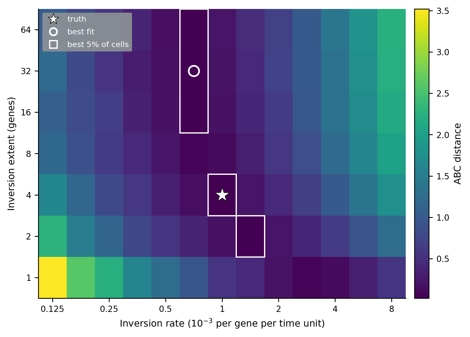
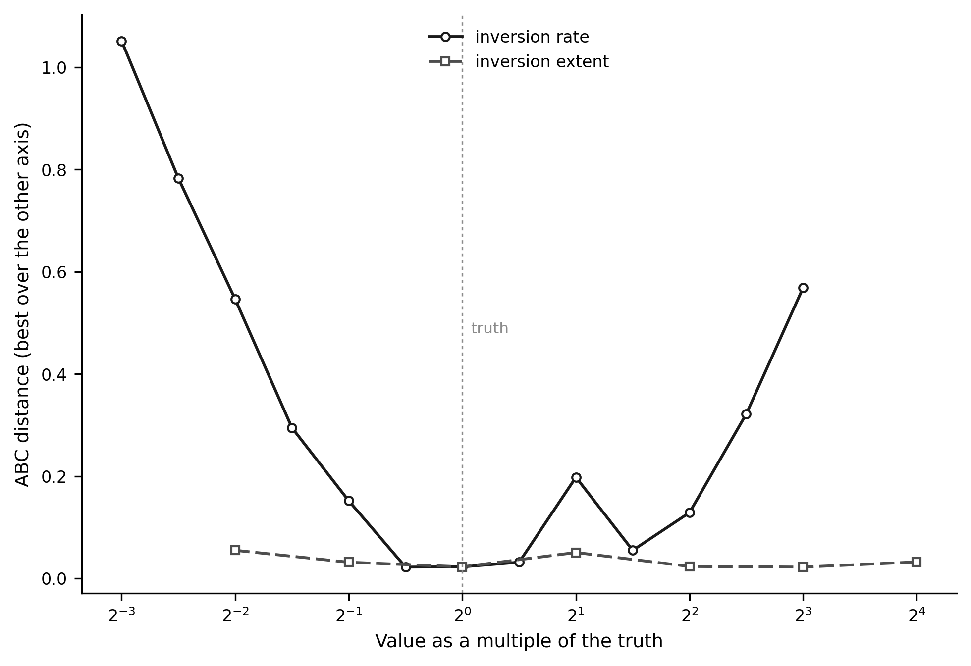
With inversions only, the ABC distance surface has a sharp valley along the rate axis and a flat ridge along the extent axis. The inversion rate comes back within one grid step of the truth in every replicate. The mean extent does not come back at all: its credible interval covers the entire grid, from 1 gene to 64 genes. Profiled along each axis, the distance moves 31 times more when the rate changes than when the extent does. Gene order tells you how often inversions happen; it does not tell you how big they are.

Two event types: both rates come back, and the mixture is real

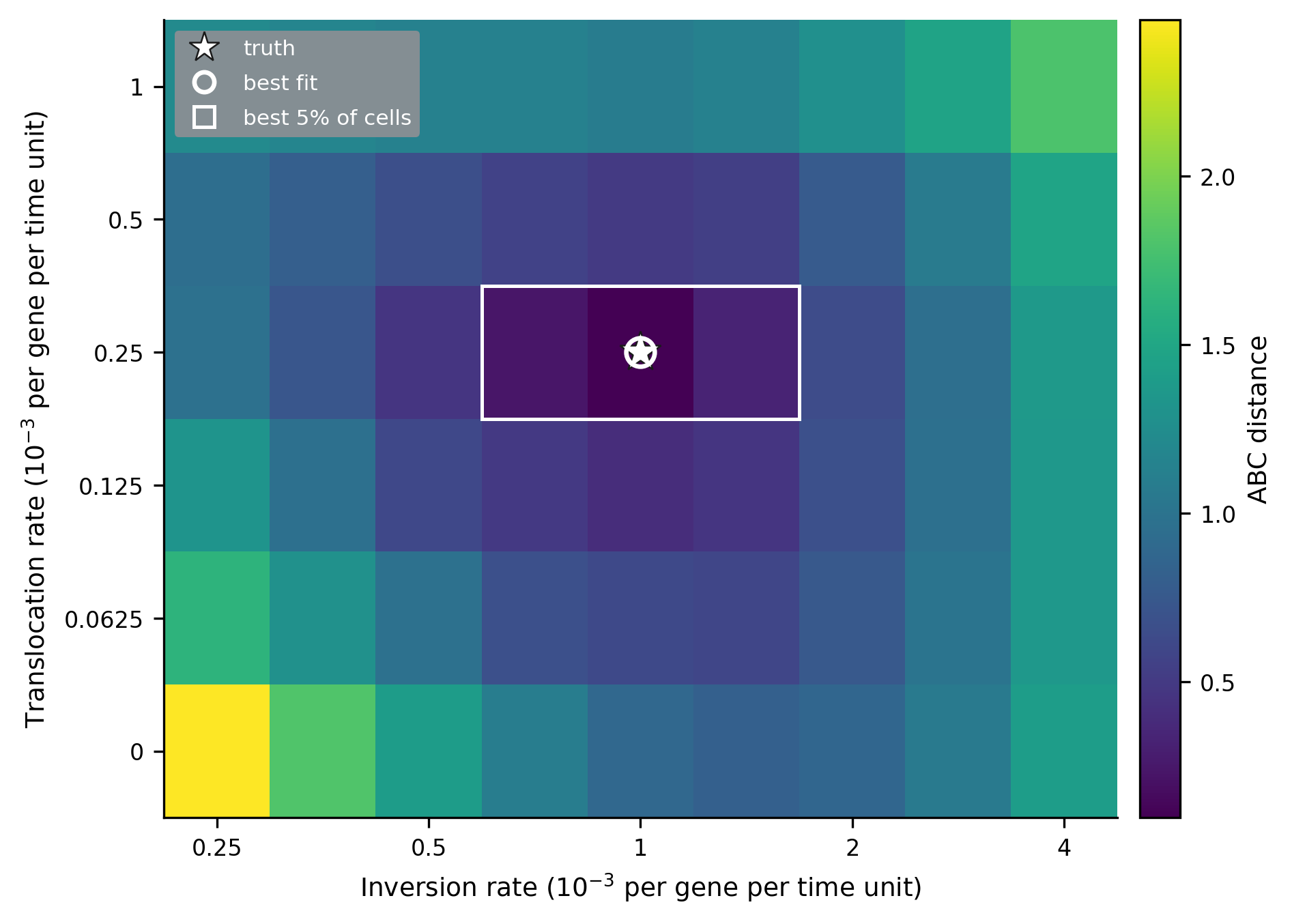
In the mixed arm the method recovers everything it is asked for, exactly, in all three replicates: the inversion rate, the translocation rate, and the 0.20 translocation share. The data also reject the simpler model rather than merely tolerating the mixture: the best inversion-only cell sits 8.2 times further from the mixed data than the best mixed cell. The statistic behind that separation is clean by construction, since cross-chromosome breaks read exactly zero when only inversions act.

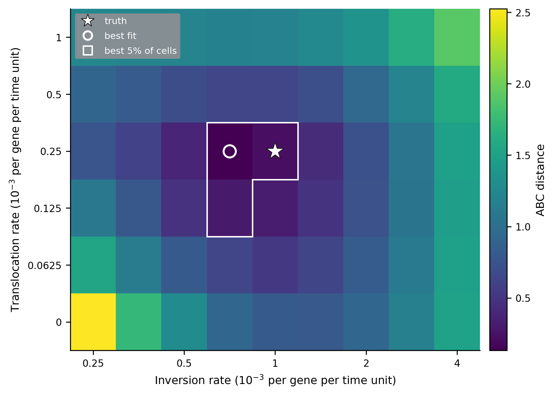
One expectation failed, and the failure is the most practical lesson in the study. Fixing the inversion extent at the wrong value, twice the truth, is not harmless: it pulls the inversion rate 29% low and inflates the apparent translocation share from 0.20 to 0.26, while leaving the translocation rate exact. A parameter the data cannot identify can still distort the ones they can.

Why ABC, and why the breakpoint distance

For an inversion-only model the likelihood is not out of reach, and this study does not claim otherwise: Caprara and Lancia (2000) analysed sorting by reversals experimentally and statistically, and York, Durrett and Nielsen (2002; 2007) built Bayesian samplers that estimate inversion counts, the 2007 version with variable tract lengths. If the question were only about inversions, one of those would be the sharper tool. The case for approximate Bayesian computation is the mixed arm: once translocations act alongside inversions, the distance and likelihood machinery developed for pure reversal models no longer applies, and ABC needs only a simulator that produces both event types and a summary statistic that keeps its meaning under both.

The breakpoint distance is that statistic, and it is worth saying plainly why it is used instead of the inversion distance. Not because it is cheaper, and not because it holds out longer: both are monotone in the number of events, both cost time linear in the number of genes, and of the two it is the inversion distance that saturates later. The reason is that the breakpoint distance counts broken adjacencies whatever broke them, so it keeps its meaning when the event model is mixed, which is exactly the regime this study targets.

References. Caprara A, Lancia G. 2000. Experimental and statistical analysis of sorting by reversals. In: Sankoff D, Nadeau JH, editors. Comparative Genomics. Dordrecht: Springer. p. 171–183. · York TL, Durrett R, Nielsen R. 2002. Bayesian estimation of the number of inversions in the history of two chromosomes. Journal of Computational Biology 9:805–818. · York TL, Durrett R, Nielsen R. 2007. Dependence of paracentric inversion rate on tract length. BMC Bioinformatics 8:115.