\appendix

Rates in detail, and the Gillespie algorithm¶

Chapter 2 introduced the shape every rate takes, effective rate = scope(base) × modifiers. This appendix is the full reference: how a rate's units work, the default scope at each level, the catalogue of modifiers and which levels accept them, and the Gillespie algorithm that turns rates into events.

How a rate is counted: the scope¶

A rate always has units of time⁻¹, on the scale imposed by the species tree. In a phylogenetic context, though, a single global rate rarely makes sense for most events. A substitution happens at a site, so a mutation rate is counted per site (mutations × time⁻¹ × per site): each site is an independent chance to mutate. A speciation happens to a lineage, so the speciation rate is counted per lineage (speciations × time⁻¹ × per lineage): each branch alive is an independent chance for the tree to split. And a gene is lost one gene copy at a time, so gene loss is counted per copy (loss × time⁻¹ × per gene-copy). The unit a rate is counted in — per lineage, per copy, per site — is what we call its scope.

By default, this is the scope ZOMBI2 uses at each level:

Level	Counted per	The rates it applies to
Species	lineage	`birth`, `death`
Genomes	copy	`duplication`, `transfer`, `loss`
Genomes	lineage	`origination`
Genomes, ordered	chromosome	`inversion`, `transposition`, `fission`, `fusion`, `chromosome_loss`
Sequences	site	`substitution` (times a clock)
Traits	lineage	`rate` (continuous), `switch` (discrete)

A bare number takes the default. To count a rate some other way, wrap it in the scope you want:

from zombi2 import species
from zombi2.rates import scope

# a death rate applied to the whole tree at once, not once per lineage
species.simulate_species_tree(birth=1.0, death=scope.Global(0.3), total_time=8.0, seed=2)

The wrappers are Global, PerLineage, PerCopy, PerSite and PerChromosome. Global(x) is the one that most changes behaviour: it detaches the rate from the amount of material present, so a Global death rate does not grow as the tree does.

Bending a rate: modifiers¶

A modifier alters a rate in context. You might give a gene family a constant loss rate across the tree except in one clade known to shed genes — a symbiotic bacterium — by multiplying the rate there. Or let families evolve at different speeds: an antimicrobial-resistance family prone to transfer, a ribosomal-protein family the opposite.

The modifiers are:

Modifier	What it does to the rate
`OnTime`	Follows a time schedule: one factor up to a breakpoint, another after it.
`OnTotalDiversity`	Slows as the tree fills up: the factor falls from 1 toward 0 as the number of lineages approaches a carrying capacity, and stays there.
`FromParent`	Is inherited from the parent lineage and nudged at each split, so the rate drifts gradually down the tree and close relatives keep similar rates.
`ByLineage`	Is an independent draw for each lineage, with no memory of its parent, so nearby branches are no more alike than distant ones.
`DrivenBy`	Reads another level: the factor is looked up from a driver's state, which is how one level conditions another (Chapter 9).

The first two are deterministic: OnTime and OnTotalDiversity are fixed functions of the state of the world, so every lineage that meets the same time, or the same diversity, gets the same factor. The next two are random and vary from lineage to lineage, and they differ in memory: FromParent is passed down and drifts, so the rate is autocorrelated along the tree — a slowly wandering clock, or a clade that inherits a fast tempo — whereas ByLineage is drawn afresh on every branch, so the variation is scattered, an uncorrelated ("relaxed") clock. The random modifiers are mean-corrected, meaning their factors average to 1, so switching on heterogeneity spreads a rate around without secretly speeding the whole tree up. DrivenBy is neither: its factor is whatever the driver's state says it is.

Modifiers stack by multiplication, so they combine: 1.0 * mod.OnTime({0: 1, 5: 0.3}) * mod.FromParent(spread=0.3) is a rate that both follows a schedule and drifts between lineages.

Which level accepts which¶

A modifier only makes sense where the level can act on it, and a level rejects a modifier it does not wire rather than silently ignoring it. This is what each accepts today:

Level	The modifiers it accepts
Species	`OnTime` · `OnTotalDiversity` · `FromParent`
Genomes	`OnTime` · `DrivenBy`
Sequences	`ByLineage`
Traits	`OnTime` · `OnTotalDiversity` · `FromParent`

The gaps are the rebuild, not the design: a level gains a modifier when its engine learns to read it. Pass one that a level does not wire and you get an error naming the modifiers that level accepts, so the table above is always recoverable from the tool itself.

The Gillespie algorithm¶

Almost every simulation here comes from one small engine, run over and over: the same loop grows a birth–death tree, duplicates and loses genes, and switches a discrete trait between states, given a different list of events each time.

That engine is the Gillespie algorithm (Gillespie 1976; Gillespie 1977), an exact, event-by-event recipe for a continuous-time process defined by rates. This section builds it from scratch — what a rate is, why waiting times are exponential, how competing events race, and how those assemble into the loop — assuming no prior exposure to continuous-time Markov chains. Rates in, a timed history out.

From a rate to a waiting time¶

A rate says how fast something tends to happen: the expected number of events per unit of time. If a gene copy is lost at rate $\mu = 0.25$, then, left alone, it is lost on average once every $1/0.25 = 4$ time units.

More precisely, a rate $\lambda$ is defined by what happens over a very short slice of time $\Delta t$. The chance that one event fires during that slice is proportional to its length,

\[P(\text{an event in the next } \Delta t) \approx \lambda\,\Delta t,\]

and the shorter the slice, the better the approximation. Notice this says nothing about a clock ticking down to the next event: in any instant the chance of firing is the same regardless of how long we have already been waiting. A rate has no memory. That single fact is what makes the whole algorithm work.

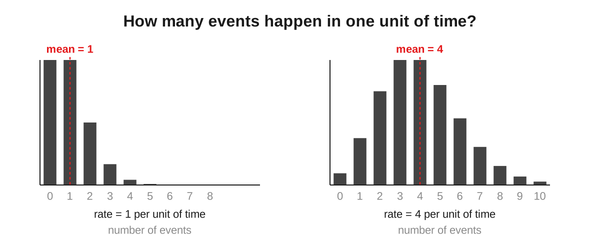
It also means a rate is a statement about probability, not a fixed schedule. A loss rate of one per unit of time does not deliver exactly one loss in every unit: over any given unit the number of events that fire is random. That count follows the Poisson distribution, with mean $\lambda T$ over an interval of length $T$ (Figure A.1).

$The count of events in a fixed window is random, not fixed. With rate $\lambda$, the number of events in one unit of time is Poisson-distributed with mean $\lambda$ (dashed line). At a low rate (left) most windows see zero or one event and a few see more; at a higher rate (right) the count spreads out around the mean. The rate fixes only the average.$

Now fix a single event with a constant rate $\lambda$ and ask: starting now, how long until it fires? Call that waiting time $W$. Because the chance of firing in each little slice is $\lambda\,\Delta t$ and slices are independent, the chance of surviving without an event up to time $t$ decays to an exponential:

\[P(W > t) = e^{-\lambda t}.\]

$W$ follows an exponential distribution with rate $\lambda$, whose mean is $1/\lambda$. Short waits are the most common. Because the exponential is memoryless, we never have to simulate the empty time between events tick by tick — we can draw the waiting time in one shot and jump to the next event. Drawing it is a single line: given a uniform random number $u$ on $(0, 1)$,

\[\Delta t = -\frac{\ln u}{\lambda},\]

which is what rng.exponential(1 / lambda) returns, its argument being the mean. Every waiting time in ZOMBI2 is drawn this way.

When several things can happen: the race¶

A real simulation never has just one possible event. A genome with many gene families can duplicate any of them, transfer any of them, or lose any of them; a species tree with many lineages can speciate or go extinct on any branch. At a given moment there is a whole menu of possible events, event $i$ with its own rate $r_i$.

Treat every possible event as an independent alarm clock, each set to go off after its own exponential waiting time. They all start together and race; the first alarm to ring is the event that happens. Two facts govern that race, and together they are the Gillespie algorithm.

When does the first event fire? The minimum of independent exponential waiting times is itself exponential, with a rate equal to the sum of the individual rates. So with a total rate

\[R = \sum_i r_i,\]

the time to the next event — whichever it turns out to be — is a single exponential draw with rate $R$. More possible events, or faster ones, means a larger $R$ and therefore shorter waits. This is why we need only one waiting-time draw per step, however long the menu.

Which event fires? The winner is event $i$ with probability equal to its share of the total rate,

\[P(\text{event } i \text{ fires}) = \frac{r_i}{R},\]

and which event wins is independent of when it happens. So the two are decided separately: draw the time from the total rate, then pick the event on a weighted roulette wheel, each slice sized to a rate.

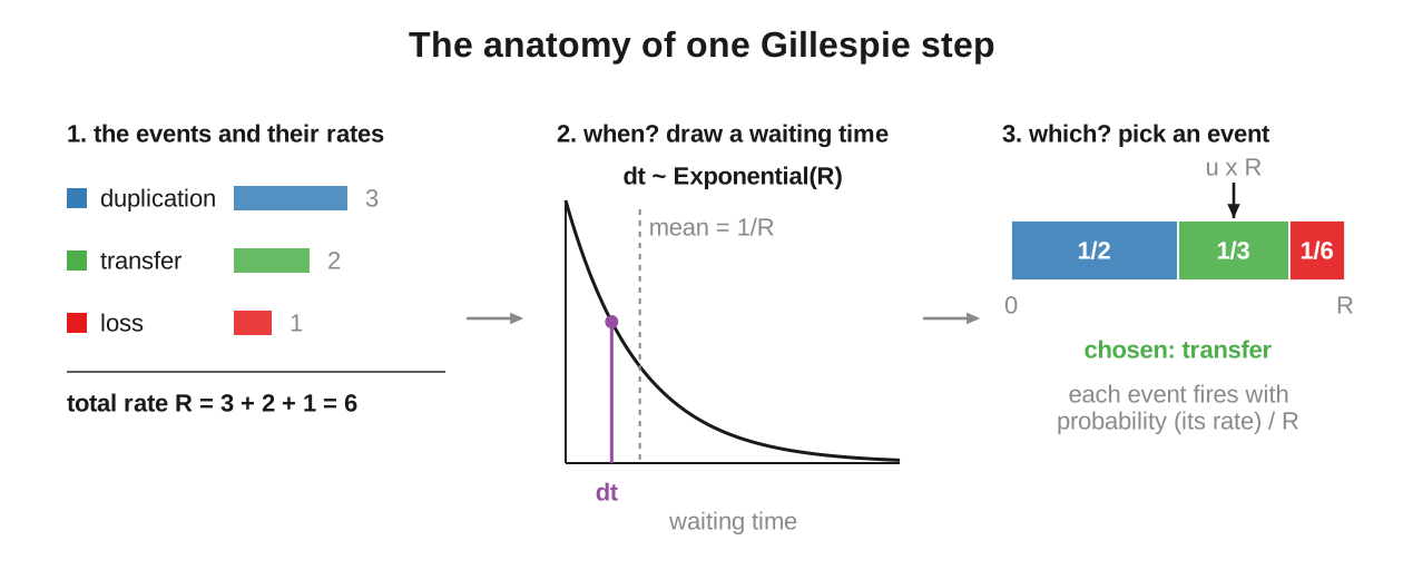
$The two draws that make up one Gillespie step. **(1)** Each possible event has a rate; here duplication, transfer and loss have rates 3, 2 and 1, summing to a total rate $R = 6$. **(2)** The waiting time to the *next* event is a single exponential draw with rate $R$; larger total rates give shorter waits, with mean $1/R$. **(3)** Which event fires is a second, independent draw: event $i$ wins with probability $r_i/R$ — the rates laid end to end as a roulette wheel, here landing on transfer. The step then advances the clock by $\Delta t$, applies the chosen event to the state, and repeats.$

In code the roulette wheel is a running sum: lay the rates end to end, draw a point uniformly along their combined length $R$, and see which segment it lands in.

The loop¶

Assembling the pieces gives the loop below. Starting from an initial state at time $t = 0$, repeat: read off the current rates and their total $R$; draw a waiting time and advance the clock; stop if the clock has run past the target time, or the process has died out; otherwise pick one event in proportion to its rate, apply it to the state, record it, and go round again.

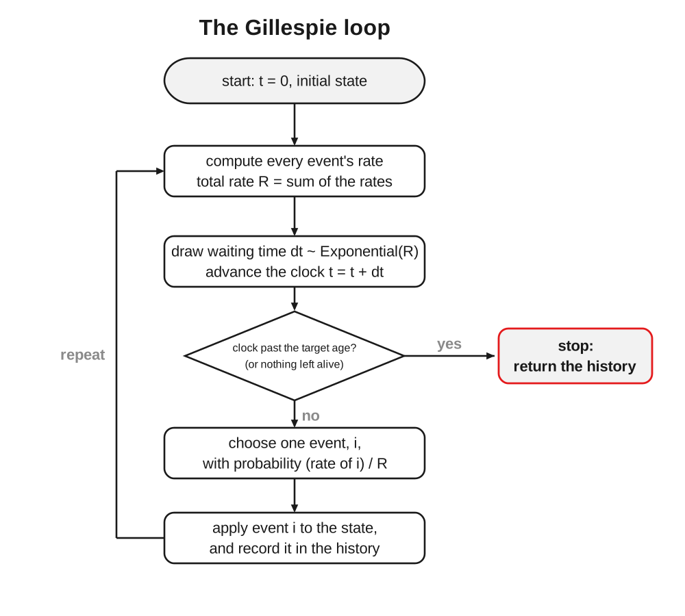
The Gillespie loop. Each pass computes the current total rate, draws one exponential waiting time, and — unless the clock has passed the target age — fires a single event chosen in proportion to its rate, updates the state, and repeats. The output is a list of events with the exact times at which they occurred: a timed history.

As pseudocode, the whole engine is short:

t = 0.0
state = initial_state
history = []
while t < total_time:
    rates = event_rates(state)      # every possible event's rate, given the state
    R = sum(rates)                  # the total rate
    if R == 0:                      # nothing can happen; the process is frozen
        break
    t += rng.exponential(1 / R)     # WHEN: draw the waiting time, advance the clock
    if t >= total_time:
        break                       # the next event would fall past the horizon
    i = choose(rates, R, rng)       # WHAT: pick an event with probability r_i / R
    state = apply(state, i)         # update the state
    history.append((t, i))          # record the timed event

The result is not a snapshot but a timed history: the exact sequence of events and the exact real-valued times at which they happened. That is what a phylogenetic simulator needs — a species tree is the history of its speciation and extinction events, a gene family is the history of its duplications, transfers and losses. Because the times are drawn from continuous exponentials rather than stepped through a fixed grid, the histories are exact: no time-step to tune, and no discretisation error.

Note

The rng is a seeded numpy random generator. Because the waiting times and event choices are its only source of randomness, the same seed reproduces the same history exactly. The clean core runs this loop in plain Python.

When the rate changes with the clock¶

The loop above assumes the rates hold still between events, so that a single $\text{Exponential}(R)$ draw lands exactly on the next event. That holds whenever the rates depend only on the current state, which changes only when an event fires. But some rates move with the clock itself, even while nothing is happening: an OnTime schedule steps at fixed breakpoints, a scheduled mass extinction arrives at a set time, and under DrivenBy the driving level changes state on its own timetable. Now $R$ is a moving target, and a draw at today's $R$ would be wrong.

ZOMBI2 keeps the draw exact by never letting it cross a change. Every rate can report the next time it changes on its own, and the engine takes the earliest such time — together with the next scheduled pulse and the end of the run — as a horizon:

Compute $R$ from the rates as they stand, and the horizon.
Draw $\Delta t \sim \text{Exponential}(R)$.
If the event lands before the horizon, fire it: the rates really were constant over that stretch, so the draw is exact.
If it lands after, discard it, advance the clock to the horizon, and start again with the rates as they are there.

Discarding is sound for the same reason the loop works at all: the exponential is memoryless, so a partial wait carries no information into the next stretch. The rates are piecewise constant, each piece gets its own exact draw, and no integral or rejection step is ever needed.

It's all Gillespie¶

Each level supplies its own events and rates, and the same loop realises all of them:

Level	The events	Their rates
Species	speciation, extinction	`birth`, `death`, per lineage
Genomes	duplication, transfer, loss, origination	one rate per event
Traits (discrete)	switches between character states	the entries of the switch matrix

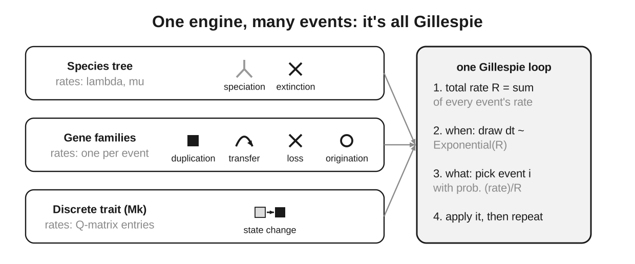
One engine, many events. Each level supplies its own events and rates, but all are realised by the identical loop on the right: total rate, exponential waiting time, an event chosen in proportion to its rate, apply, repeat.

Swapping levels swaps the list of events and how their rates are computed; the timing machinery — total rate, exponential wait, proportional choice — never changes.

…except when it isn't¶

ZOMBI2 steps outside the event-by-event loop in two places, for the same reason both times: when only the endpoints are needed, not the whole timed history, an exact shortcut beats simulating events you would throw away.

The first is sequence substitution along a branch. Once a gene tree and its branch lengths are settled, evolving a sequence down a branch does not require the individual substitution events, only the state at each end. The probability of ending in each state after a branch of length $t$ is given exactly by the matrix exponential $P(t) = e^{Qt}$, so ZOMBI2 draws each site's descendant state straight from $P(t)$ in one step (Sequence evolution). Running Gillespie here would generate, and then discard, thousands of intermediate substitutions.

The second is a continuous trait. Brownian motion has no events to fire — it moves at every instant — so there is nothing for the loop to enumerate. A constant-rate run is drawn in closed form instead, as one multivariate normal over the whole tree, with variance $\sigma^2 \times$ root-to-tip depth and covariance $\sigma^2 \times$ shared path length (Trait evolution). When the rate varies along the tree, each branch takes the exact integral of $\sigma^2$ over it.

The rule of thumb is the same each time. Reach for Gillespie when you need the whole history — every branching, gain and loss at its exact time; reach for a shortcut when the endpoints are all you need. For the trees and genomes that are ZOMBI2's real subject the history is the result, so the loop is the norm and these two shortcuts are the exceptions.